Opening the Black Box: A Look Inside Core Explainable AI Techniques
The version of 'HOW'

Introduction: From 'Why' to 'How'
In the first part of our journey into Explainable AI (XAI), we established the critical need to move beyond opaque "black box" systems. We explored the risks associated with AI we don't understand – risks to trust, fairness, safety, and compliance. Now, we shift focus from the why to the how. If we need to understand AI decisions, what tools and techniques actually allow us to do that?
Welcome to the XAI toolbox. This isn't a single magic wand, but rather a diverse set of methodologies developed to shed light on complex models. Some tools offer a wide-angle view of a model's general behavior, while others provide a magnifying glass to examine individual predictions. In this article, we'll unpack some of the most prominent techniques, focusing particularly on two influential methods – LIME and SHAP – and exploring the broader landscape of explainability approaches.
Section 1: The Landscape of Explainability Methods – Navigating the Options
Before diving into specific tools, it's helpful to understand some key ways XAI techniques are categorized:
Model-Specific vs. Model-Agnostic: As mentioned briefly before, this is a crucial distinction. Model-specific methods exploit the internal architecture of particular model types (e.g., calculating feature importance directly from tree structures in Random Forests, or examining weights in linear models). They can be very efficient and precise if your model type is supported. Model-agnostic methods, however, treat the AI model as an opaque box. They work by systematically changing inputs and observing the corresponding changes in outputs, allowing them to be applied to virtually any model (from complex neural networks to ensemble methods). This flexibility is a major advantage.
Local vs. Global Explanations: Does the explanation focus on a single prediction or the model's overall behavior? Local explanations aim to justify why the model made a specific decision for a particular input instance (e.g., why this loan application was denied). Global explanations seek to understand the model's general tendencies and the average influence of features across the entire dataset (e.g., what factors does the model generally consider most important for loan approval?). Both perspectives are vital for a complete understanding.
Intrinsic vs. Post-Hoc Explainability: Intrinsic explainability refers to using models that are understandable by their very nature (like simple decision trees or linear regression). Post-hoc explainability involves applying techniques after a model (often a complex black box) has been trained to understand its behavior. Much of the focus in XAI, especially when dealing with state-of-the-art performance models, lies in developing effective post-hoc methods. Our focus today is primarily on post-hoc, model-agnostic techniques.
Section 2: Deep Dive: LIME (Local Interpretable Model-agnostic Explanations)
LIME is perhaps one of the most intuitively appealing XAI techniques. Its core idea is elegantly simple: even if a complex model's global behavior is incredibly intricate (like a wildly curving line), its behavior very close to a specific point can often be approximated by a much simpler model (like a straight line tangent to the curve at that point).
How it Works (Conceptual):
Select Instance: Choose the specific prediction you want to explain.
Perturb: Create numerous slightly modified versions (neighbors) of this input instance. For text, this might involve removing words; for images, turning superpixels on/off; for tabular data, slightly changing feature values.
Predict: Get the original black-box model's predictions for all these perturbed neighbors.
Weight: Assign higher importance (weight) to neighbors that are very similar (proximate) to the original instance and lower weight to those further away.
Fit Interpretable Model: Train a simple, inherently interpretable model (commonly a weighted linear model) on this local dataset of neighbors and their predictions.
Explain: The parameters of this simple local model (e.g., the feature weights in the linear model) serve as the explanation for the black-box model's prediction for the original instance. They show which features locally contributed positively or negatively to the outcome.
Strengths: Its main strength is its model-agnosticism – it can be applied to virtually any classifier or regressor. The explanations are local and relatively intuitive, focusing on the factors driving a single decision.
Weaknesses: Explanations can sometimes be unstable – slightly different sets of perturbations might lead to different explanations. Defining the 'locality' (how neighbors are generated and weighted) can be challenging and affect the outcome. Its explanations are primarily local, offering limited insight into the model's global behavior.
Section 3: Deep Dive: SHAP (SHapley Additive exPlanations)
SHAP brings a more rigorous, theoretically grounded approach derived from cooperative game theory. The central concept is the Shapley value, developed by Nobel laureate Lloyd Shapley. In game theory, it provides a unique, fair way to distribute the total 'payout' of a cooperative game among its players based on their individual contributions to all possible coalitions (teams).
How it Works (Conceptual):
Analogy: Think of the 'game' as the model's prediction task. The 'players' are the input features. The 'payout' is the difference between the model's actual prediction for an instance and a baseline prediction (e.g., the average prediction across the dataset).
Contribution: SHAP calculates the Shapley value for each feature. This value represents that feature's average marginal contribution to the 'payout' across all possible combinations (coalitions) of other features. Essentially, it asks: "How much does knowing the value of this specific feature change the expected prediction, considering all contexts?"
Computation: Calculating exact Shapley values is computationally exponential. Therefore, practical SHAP implementations (like KernelSHAP, TreeSHAP, DeepSHAP) use clever approximations or model-specific optimizations to estimate these values efficiently.
Explanation: The resulting SHAP values for an instance provide a local explanation, showing the positive or negative contribution of each feature to that specific prediction. Crucially, these local values can be aggregated to generate powerful global explanations.
Strengths: SHAP has a strong theoretical foundation based on fairness axioms (e.g., Efficiency, Symmetry, Dummy, Additivity), ensuring a principled distribution of contribution. It provides both local and global explanations (feature importance rankings, feature dependence plots, interaction effects). SHAP values are generally considered more stable and consistent than LIME explanations.
Weaknesses: It can be computationally more intensive than LIME, especially the model-agnostic KernelSHAP variant. The interpretation of Shapley values, while powerful, requires a bit more understanding than simple linear weights. Some SHAP implementations make simplifying assumptions (like feature independence) that might not always hold true.
Section 4: LIME vs. SHAP – A Practical Comparison
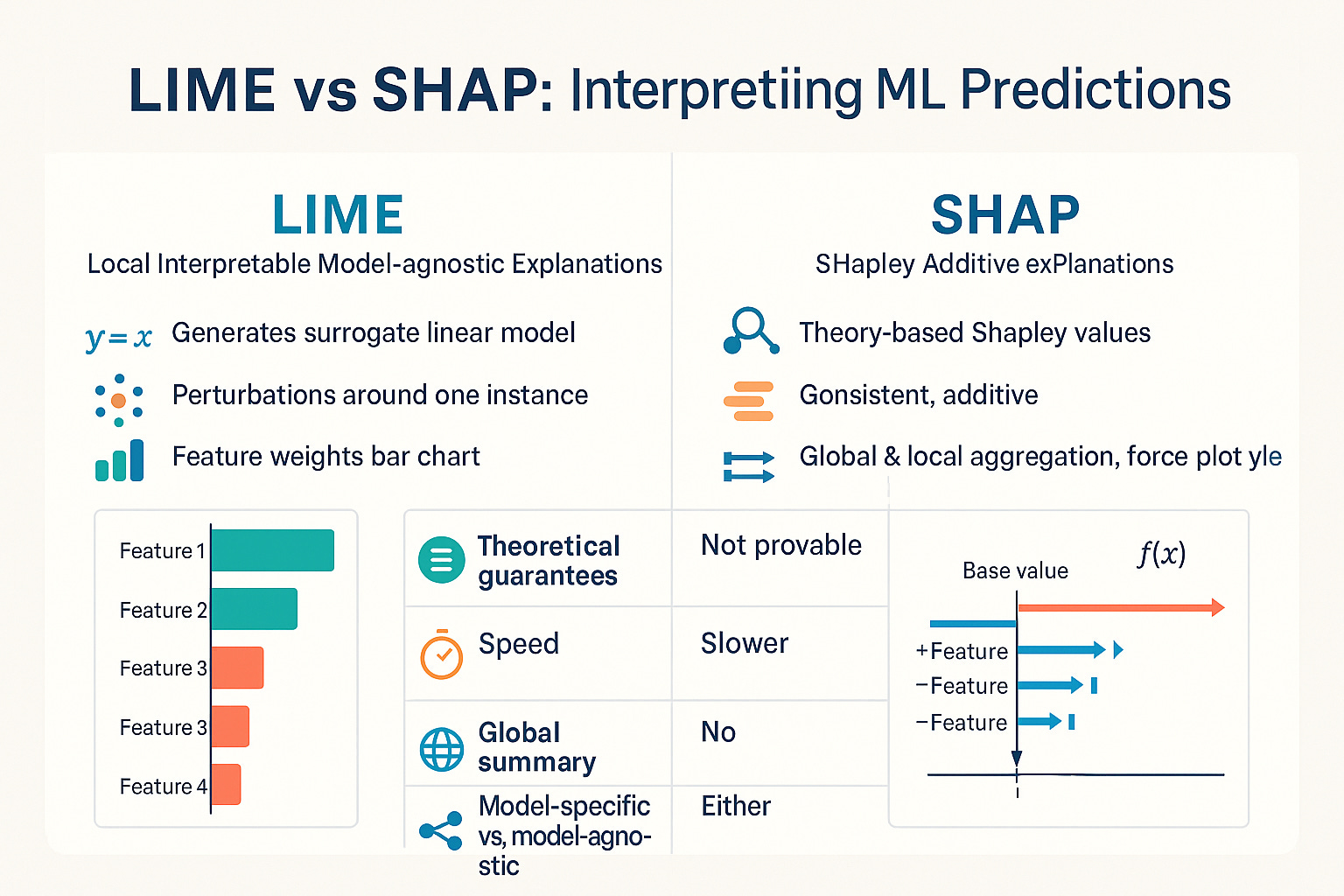
Feature LIME SHAP Core Approach Local linear approximation via perturbation Game theory (Shapley values) via contribution Model Type Model-Agnostic Model-Agnostic (KernelSHAP) & Specific Variants Explanation Type Primarily Local Local & Global Stability Can be less stable Generally more stable Computation Often faster Can be slower (esp. KernelSHAP) Theory Heuristic-based Strong theoretical grounding (Shapley axioms) Output Local feature weights/importance Additive feature attributions (local/global)
When to prefer LIME? When you need quick, intuitive local explanations for any model type and computational speed is a priority, or if the theoretical guarantees of SHAP are less critical for your specific use case.
When to prefer SHAP? When you need robust, theoretically sound explanations, desire both local and global insights, require more stable explanations, or are using models where efficient SHAP variants (like TreeSHAP) are available.
Section 5: Beyond LIME and SHAP – Other Tools in the Box
While LIME and SHAP are highly influential, the XAI toolbox contains many other valuable techniques:
Global Feature Importance: Methods like Permutation Feature Importance assess how much a model's overall performance drops when the values of a specific feature are randomly shuffled, indicating its importance.
Partial Dependence Plots (PDPs) & Accumulated Local Effects (ALE) Plots: These visualize the average relationship between a feature (or two features) and the model's prediction, helping understand marginal effects globally. ALE plots are often preferred as they handle correlated features better than PDPs.
Rule-Based Explanations: Techniques like Anchors or rule extraction algorithms aim to find simple IF-THEN rules that locally (or sometimes globally) explain the model's predictions.
Gradient-Based Methods (for Deep Learning): Techniques like Saliency Maps, Integrated Gradients, Grad-CAM, and Layer-Wise Relevance Propagation (LRP) are designed specifically for deep neural networks, often highlighting which input pixels (for images) or words (for text) were most influential.
The choice of technique depends heavily on the type of model, the data, the specific question being asked, and the target audience for the explanation.
Conclusion: Choosing the Right Lens
Opening the AI black box isn't about finding one single key, but rather about having a versatile set of tools and knowing when and how to use them. Techniques like LIME and SHAP provide powerful lenses for examining model behavior, offering crucial local and global insights that were previously inaccessible for complex systems. They represent significant steps towards building more transparent, trustworthy, and accountable AI.
However, as we'll explore in the next segment, these tools are not without their own limitations and challenges. Understanding how these explanations are generated is the first step; critically evaluating their meaning, scope, and potential pitfalls is the essential next one.
Which XAI techniques have you encountered or found most useful? What challenges have you faced in trying to explain AI models? Share your insights in the comments!
Stay tuned for Segment 3, where we delve into the limitations and trade-offs of XAI. Subscribe to ensure you don't miss it: